In part 1 of this series I discussed downloading and installing the R statistical package and loading it with Howard County election data, and then in part 2 we began to explore how to use that data to estimate the percentages of voters in the 2010 general election who are Democrats, Republicans, or unaffiliated or members of other parties. In our initial explorations we discovered that the percentage of those voting who were Republicans seemed to be relatively static over the years.
Now it’s time to continue our exploration, this time looking at the historical data for the percentage of voters who were Democrats or unaffiliated or other. Let’s repeat what we did for the Republican data, plotting the percentage of Democratic voters hgg$PctVotersD over the years:
> plot(hgg$Year, hgg$PctVotersD)
>
The resulting graph shows a clear downward trend over the years:
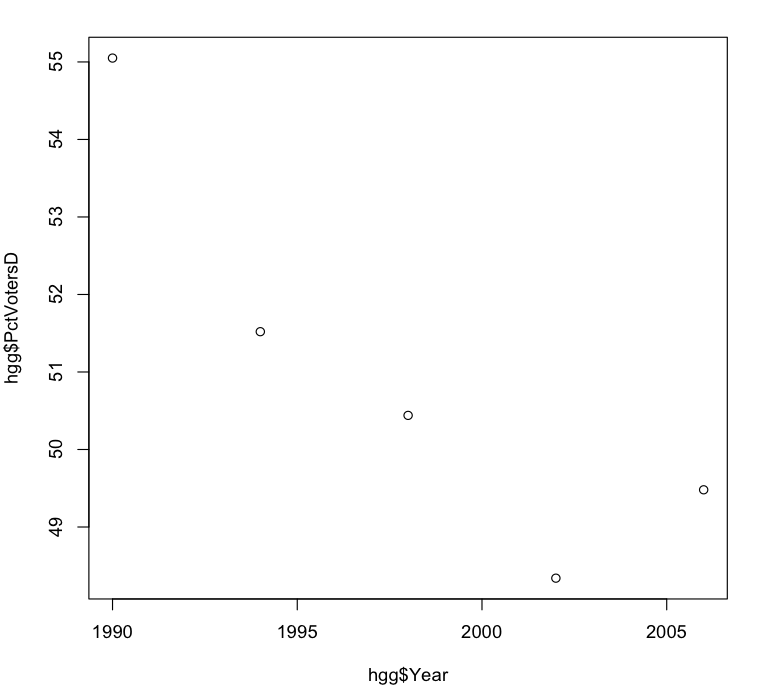
This might seem surprising in combination with the graph in the previous post showing that the Republican share of total voters has remained relatively stable over the years. Given that Democratic registration in Howard County has supposedly been outpacing Republican registration by a considerable margin, shouldn’t the percentage of Democratic voters be trending upward over the years, and the percentage of Republican voters trending downward?
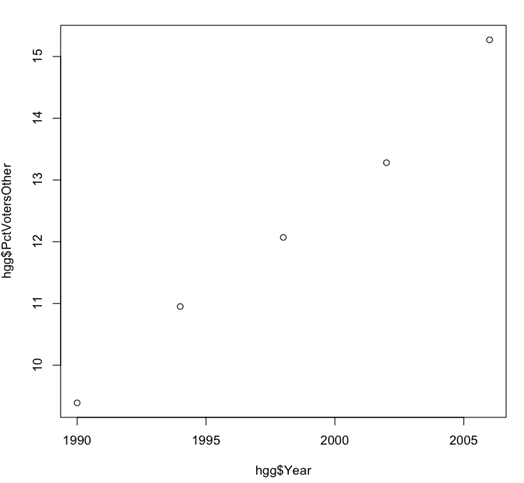
Part of the answer may lie in the difference between registering voters and having those voters actually turn out for elections. However another part of the answer lies in the role of unaffiliated and other voters. Let’s plot the percentage of unaffiliated and other voters hgg$PctVotersOther for comparison:
> plot(hgg$Year, hgg$PctVotersOther)
>
The resulting graph shows a clear and (at first glance) almost perfectly linear upward trend in the percentage of people voting who are unaffiliated or belong to other parties.
So possibly what’s happening is that the rising percentage of unaffiliated and other voters is cutting into the Democratic fraction of voters more than into the Republican fraction.
But that’s a question for another day. For now let’s continue with trying to estimate the various percentages of voters for each party and for independents. To help us do that, let’s plot all the values in one graph. We’ll start with a plot like the one we did for Republican voters in the previous post, and then add to it the values for Democratic voters and for unaffiliated and other voters:
> plot(hgg$Year, hgg$PctVotersR, xlim=c(1990, 2010), ylim=c(0, 60))
> points(hgg$Year, hgg$PctVotersD)
> points(hgg$Year, hgg$PctVotersOther)
>
Note that as in the original plot we set the vertical or “y” axis to go from 0 to 60%. In this new plot we also use the xlim parameter to set the horizontal (“x”) axis to go from 1990 to 2010, in order to help us envision how the historical trends might project forward to this year. To the graph produced by plot() we then add points for hgg$PctVotersD and hgg$PctVotersOther, both plotted against hgg$Year. (Note that the points() function does not start a brand-new graph, but simply overlays new data points on the graph already being displayed.)
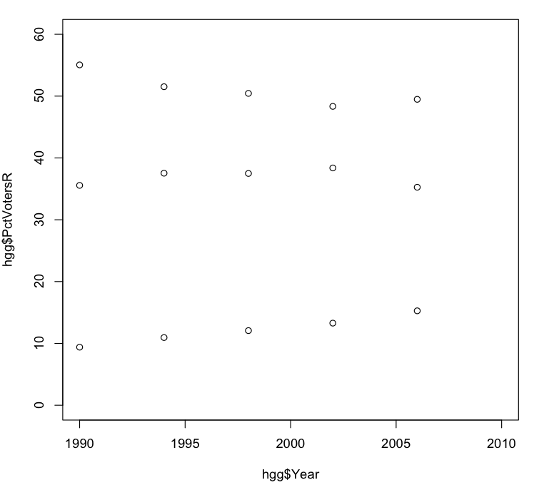
From the above graph we can do a quick eyeball estimate of where the percentages of voters might end up in 2010, assuming historical trends continue. The percentage of unaffiliated voters looks like it might be around 17-18%, and the percentage of Democrats around 47-48%; that would leave the percentage of Republican voters around 35% or so.
However with R we can produce a more exact prediction by creating a “linear model” of the data. In a linear relationship change in one variable is associated with a proportional change in another variable. For example, based on the data for hgg$PctVotersOther:
> hgg$PctVotersOther
[1]  9.39 10.95 12.07 13.28 15.27
>
an increase of four years (i.e., between elections) appears to be associated with an increase of over 1% in the percentage of unaffiliated and other voters, or about a quarter to a third of a percent per year. To get a more exact estimate we use the lm() function:
> lm(hgg$PctVotersOther ~ hgg$Year)

Call:
lm(formula = hgg$PctVotersOther ~ hgg$Year)

Coefficients:
(Intercept)     hgg$Year
  -691.6035       0.3522

>
Here lm() tries to find a linear relationship between hgg$PctVotersOther and hgg$Year, such that given a value of hgg$Year we can predict a corresponding value for hgg$PctVotersOther. This produces two numbers of interest. The first number, 0.3522, is the estimated increase per year in the percentage of unaffiliated and other voters. (This is known as the “slope” of the line.)
The second number, -691.6035 (known as the “intercept”), is the value that hgg$PctVotersOther would have if we projected back to hgg$Year having a value of zero. Of course this doesn’t make sense in real life, but simply serves to help calculate estimated values of hgg$PctVotersOther. For example, if hgg$Year has the value 1990 then we calculate the estimated value of hgg$PctVotersOther in that year by multiplying the slope value (0.3522) by 1990 and then adding the intercept value (-691.6035):
> 0.3522 * 1990 - 691.6035
[1] 9.2745
>

Compare this to the actual percentage of unaffliated and other voters in 1990, which is given by the first element of `hgg$PctVotersOther`:

```r
> hgg$PctVotersOther[1]
[1] 9.39
>
We could continue through the years, calculating estimates of hgg$PctVotersOther for 1994, 1998, and so on; since the percentage of unaffiliated and other voters doesn’t follow an exact linear trend, there will be minor differences between the estimated values and the actual values. The goal of linear modeling (as implemented by lm()) is to find a line that minimizes the total amount of those differences.1
We can show how closely that line fits the actual data by taking our plot from above and using the abline() function to add to it a line having the slope and intercept calculated above.[^2]
> abline(-691.6035, 0.3522)
>
Note that we don’t have to repeat the previous plot() and point() functions, as long as we haven’t issued a new plot() function in the meantime.
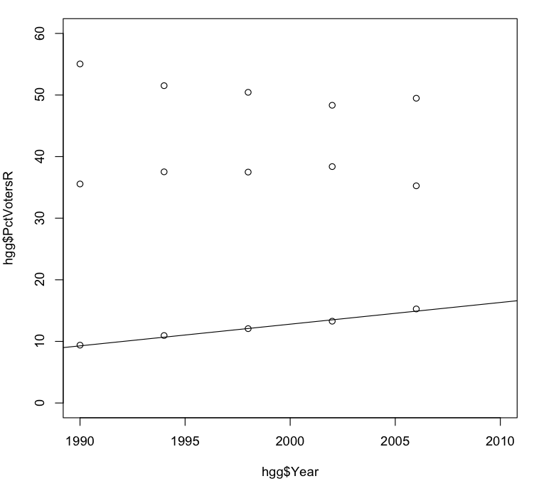
But enough of the preliminaries: Let’s make an estimate! Given the values of slope and intercept given above, we can compute the predicted percentage of unaffiliated and other voters in the 2010 general election as follows:
> 0.3522 * 2010 - 691.6035
[1] 16.3185
>
So our first prediction is that unaffiliated and other voters will be 16.3% of those voting in Howard County in the 2010 general election. I’ll continue this analysis in the next post, in which we’ll find an estimate for the proportion of Democratic voters.
[^2] The abline() function gets its name from the traditional mathematical equation for a line, $y = ax + b$, in which $x$ is a variable on which $y$ depends, $a$ is a constant value giving the slope, and $b$ is a second constant value giving the intercept.
Trevor - 2010-11-16 14:49
This is great stuff. You ever thought about a second career in polling?
hecker - 2010-11-16 15:02
I don’t think I’m cut out to be a pollster, to be honest. This is just a hobby, and I plan to keep it that way.
To be more precise,
lm()finds a line that minimizes the sum of the squares of the differences. Hence this procedure is known as least squares analysis. ↩︎